Lorenzo Alberton
« Articles
Historical Twitter access - A journey into optimising Hadoop jobs
Abstract: A journey into optimising Hadoop jobs: the strategies to scan and filter a PetaByte of archived data, schedule new jobs and deliver data fast.
A journey into optimising Hadoop jobs
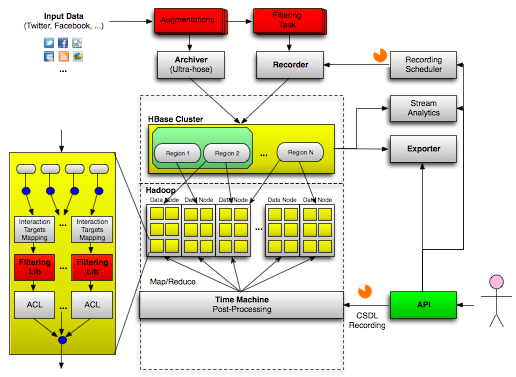
 At DataSift we are in the enviable position of receiving the full Twitter Firehose in real time (currently 400 million messages/day), plus many other data sources and augmentations. So far, we've been offering the ability to filter the messages and deliver the custom output stream in real time. Some time ago we also started recording everything on our internal Hadoop cluster, since we wanted to run analytics and offer filtering on past data too. At the current rate, we store about 2 TeraBytes of compressed data every day. As a data store, we chose HBase on HDFS because we needed random access to individual records, combined with the ability of scanning sorted sets and running complex Map/Reduce jobs.
Whilst our cluster size isn't really comparable with the largest Hadoop deployments in the medical or physics fields, at just under 1 PetaByte and doubling in size every 3 months, it's probably a lot larger than the average amount of data most companies have to deal with.
Since the announcement of our closed alpha, the demand for historical Twitter access has been huge, so we knew early on that we couldn't release a service that would collapse with just a couple of queries or that took forever to process data: if you start a query now, you don't want results in 15 days.
Getting closer to the data
Scanning the data in HDFS is quite fast, however I/O is still the biggest bottleneck, especially with HBase. Since we always strive to offer top performance, we started thinking about ways of pushing our batch Map/Reduce jobs faster and faster.
The first big improvement was to turn our filtering engine from a service into a C++ library, so we could execute custom queries locally on each node of the cluster, from within the Map task, instead of constantly moving data from the cluster to the remote service. This change alone, combined with a better serialisation format, translated into a 20x speed boost, and of course should scale more or less linearly with the number of nodes in the cluster.
Improving parallelisation
Filtering closer to the data was an improvement, but we didn't stop there. Scanning billions of records on each node means I/O still trumps CPU load by orders of magnitude, meaning we weren't making very good use of our filtering engine, which was designed to handle thousands of concurrent filters. So we had another hard look at the system to see whether we could squeeze more cycles out of those CPUs.
The idea we came up with solved several problems at once:
- parallel execution of sub-tasks
- fair queuing of scheduled jobs
- dynamic prioritisation and allocation of jobs for maximum throughput
- ability to give higher priority to certain jobs
Here's what we did.
Each historical query can be submitted at any time, and each one of them could be very different in length (some could span weeks/months of archived data, some others could be much shorter and limited to a few hours/days), making it difficult to have an optimal schedule. Once a query is started, it has to complete, and newly submitted queries cannot be executed in parallel in the same process with already running ones, even if they overlap. A long-running query could also easily occupy most of the available resources for a long time, thus starving the pending queries.
In order to maximise the execution parallelism, we needed a strategy that maximised the overlap of pending queries, and avoided allocating Map/Reduce slots to any single query for too long.
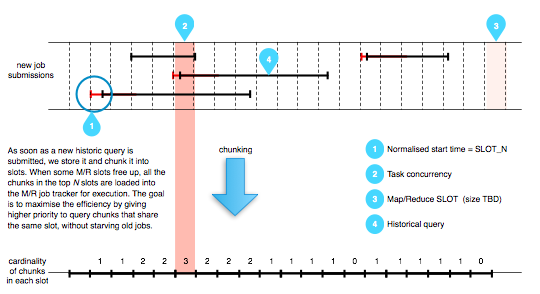
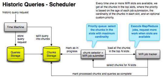
The solution to both problems was to split each query into smaller chunks, whose size was big enough to minimise the M/R job start-up overhead, but small enough to be executed within a predictable time. The query chunks are added to a queue of pending M/R tasks, and as soon as the cluster has some capacity to run more M/R jobs, the system selects the most promising chunks off the queue.
The way each job is partitioned into chunks could be done in many ways. The first attempt (chunking strategy #1) could be to chunk queries only if - at the time the pending queue is evaluated - there's an overlap, but this would likely lead to lots of chunks of widely different sizes, and to unpredictable execution times as a consequence. A better approach (chunking strategy #2) is to divide the timeline in slots of equal, predetermined size, and then to partition the queries according to the slots boundaries they fall into. Of course the overlap of chunks on a slot thus determined is not always perfect, but it's easy to skip the records outside the chunk range when the query is executed, whilst still enjoying the benefits of an easier partitioning strategy and an upper bound on the amount of work for each chunk.
Let me explain the two strategies with a diagram.
Chunking strategy #1
| Query | Time of arrival | From | To |
|---|---|---|---|
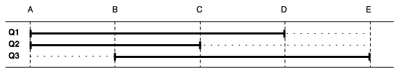
| Q1 | t | A | D |
| Q2 | t + 30m | A | C |
| Q3 | t + 45m | B | E |
Supposing for simplicity that we can only run one M/R job at the same time, and that it takes 1 hour to scan a single segment of the archive (e.g. the segment AB or BC). If at time t we receive the query Q1 and the job tracker is free, Q1 is immediately executed (as a single job), and it will take 3 hours to complete (AB + BC + CD). At time (t0 + 30m) we receive Q2 and at time (t0 + 45) we receive Q3, but both remain in the pending queue until the first job is done. At time (t0 + 3h) we can start processing the segment BC for Q2 and Q3 together; at time (t0 + 4h) we can run the segment AB for query Q2; at time (t0 + 5h) we can run the segment CE for query Q3. The total process requires 7 hours.
| Time | Pending queue | Chosen for execution | Execution time |
|---|---|---|---|
| t | Q1 (AD) | Q1 (AD)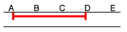 | 3 hours |
| t + 3h | Q2 (AC) Q3 (BE) | Q2 + Q3 (BC)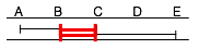 | 1 hour |
| t + 4h | Q2 (AB) Q3 (CE) | Q2 (AB)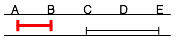 | 1 hour |
| t + 5h | Q3 (CE) | Q3 (CE)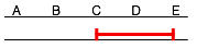 | 2 hours |
Chunking strategy #2
If now we decide to chunk every query in slots of equal size, even if there's no overlap at this time, here's what happens with the same queries as above.
At time t only query Q1 is available: its segment AB is started. At time (t + 1h) we can run the segment BC for all three queries. At time (t + 2h) we can run segment CD for queries Q1 and Q3. At time (t + 3h) we run segment AB for query Q2 and at time (t + 4h) we run the last segment DE for query Q3. The total process now only requires 5 hours, thanks to the more dynamic scheduling and to unconditional chunking into slots of predictable execution time.
| Time | Pending queue | Chosen for execution | Execution time |
|---|---|---|---|
| t | AB (Q1) BC (Q1) CD (Q1) | AB (Q1)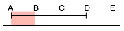 | 1 hour |
| t + 1h | AB (Q2) BC (Q1 + Q2 + Q3) CD (Q1 + Q3) DE (Q3) | BC (Q1 + Q2 + Q3)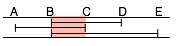 | 1 hour |
| t + 2h | AB (Q2) CD (Q1 + Q3) DE (Q3) | CD (Q1 + Q3)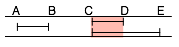 | 1 hour |
| t + 3h | AB (Q2) DE (Q3) | AB (Q2)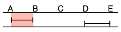 | 1 hour |
| t + 4h | DE (Q3) | DE (Q3)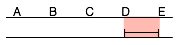 | 1 hour |
Dynamic scheduling
The last interesting characteristic of this system is the order chunks are chosen for execution, and it can be summarised as a priority queue with three parameters:
- the cardinality of each slot (i.e. how many chunks happen to be in the same slot: the higher the slot cardinality, the higher the priority given to the chunks in that slot);
- the age of each query (because we don't want to starve old queries with a low overlap cardinality);
- custom priorities (so we can tweak the priority of a single query if we need to execute it immediately).
The beauty of this strategy is that the execution priority of the pending chunks is re-evaluated every time Hadoop has spare capacity (as determined by the job monitor) to execute new jobs, for all pending chunks (and not just for pending queries as a whole) and can be maintained to a near-optimal level of parallelism at any time.
There's still some extra complexity to join chunks back into a query to determine when the original query is fully executed, but handling this is quite trivial.
The result is we can now run hundreds of concurrent queries, optimising data scans and taking full advantage of our massively-parallel filtering engine, at the data is scanned and delivered up to 100x faster than real-time.
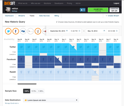
Data sampling
With such a large volume of data being produced every day, many people are not interested in receiving every single message matching a filter, a random sample of the results is more than enough, resulting in a significant saving in licensing cost. For live streams, we already offer a special predicate to select a percentage of the results, we likewise offer a 1%, 10% or 100% sample of results from the archive.
The way we implemented it is actually quite interesting too.
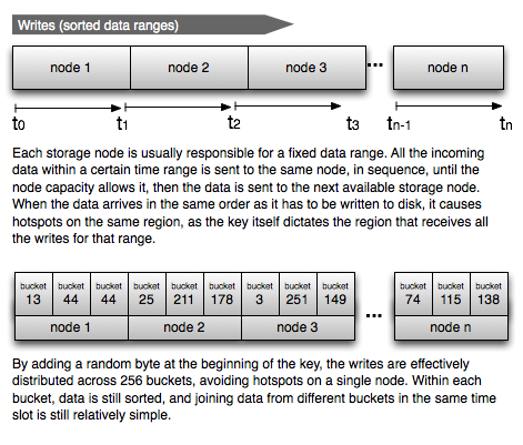
As mentioned at the beginning, we need to store the data in sequential order, so we can scan sorted time ranges. This write pattern usually creates hot spots in any cluster, be it HBase or Cassandra or another distributed database. All the data for a time range usually has to be stored in the same region to keep it sorted, and to make it possible to do range scans.
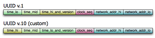
To avoid hot spots, we played a simple trick: we added a random byte in front of the row key, effectively sharding the data in 256 buckets (~20 groups). The rest of the row key contains a special UUID which is strictly time-ordered, keeping the data sorted in each bucket. When reading, we have to start 256 Map tasks for each date range we need to scan/filter, but each task is much more efficient, as the data is better distributed across all nodes in the cluster and not just in one single region.
Since each write is randomly sent to one of the 256 buckets, each bucket contains a 1/256 truly random sample over the given time range, so when you choose a sample over the archived data, we can harness this property and only read data from one or more buckets, depending on the sampling rate, with obvious gains in terms of speed and efficiency, as we don't need to scan all the data, and we don't need to start 256 map tasks. Thanks to this fact, we're happy to pass onto you both the speed gains in producing the results and a significant saving in processing cost :-)
Improving delivery
A big engineering effort also went into optimising the delivery itself: as a teaser, we parted quite drastically from the "traditional" Map/Reduce execution, improved the network layer and implemented a much better API and many new connectors, but I'll leave the details to another blog post, there's a lot to talk about :-)
Conclusion
 The last three months at work have been really intense, and as you now know they involved a lot of reengineering and re-architecting of the DataSift platform, however we're super-excited about what we achieved (I'm constantly humbled by working with such a talented team of engineers) and about finally making this service generally available to all customers.
If you've been waiting a long time for historical Twitter access, we're confident it was totally worth the wait. Happy data sifting!
Related articles
Latest articles
- On batching vs. latency, and jobqueue models
- Updated Kafka PHP client library
- Musings on some technical papers I read this weekend: Google Dremel, NoSQL comparison, Gossip Protocols
- Historical Twitter access - A journey into optimising Hadoop jobs
- Kafka proposed as Apache incubator project
- NoSQL Databases: What, When and Why (PHPUK2011)
- PHPNW10 slides and new job!
Filter articles by topic
AJAX, Apache, Book Review, Charset, Cheat Sheet, Data structures, Database, Firebird SQL, Hadoop, Imagick, INFORMATION_SCHEMA, JavaScript, Kafka, Linux, Message Queues, mod_rewrite, Monitoring, MySQL, NoSQL, Oracle, PDO, PEAR, Performance, PHP, PostgreSQL, Profiling, Scalability, Security, SPL, SQL Server, SQLite, Testing, Tutorial, TYPO3, Windows, Zend FrameworkFollow @lorenzoalberton